pde_parabolic.html

Parabolische DGl. (mit und ohne Driftterm)
(verschiedene Randbedingungen)

> restart:

> with(PDEtools):

> PDE1 := diff(u(x,t),t)=1/20*diff(u(x,t),x,x); # ohne Driftterm

> PDE2 := diff(u(x,t),t)=1/20*diff(u(x,t),x,x) + 1/2*diff(u(x,t),x); # mit Driftterm

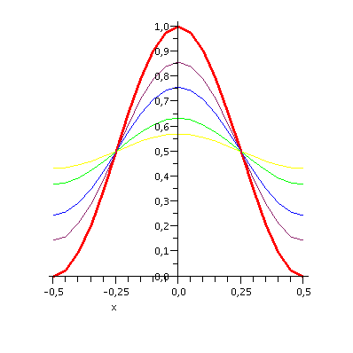
> IBC1 := {u(x,0)=cos(Pi*x)^2, D[1](u)(-1/2,t)=0,D[1](u)(1/2,t)=0}; # AB + Neumann-RB

$(Typesetting:-mprintslash)([IBC1 := {u(x, 0) = cos(Pi*x)^2, (D[1](u))((-1)/2, t) = 0, (D[1](u))(1/2, t) = 0}], [{u(x, 0) = cos(Pi*x)^2, (D[1](u))((-1)/2, t) = 0, (D[1](u))(1/2, t) = 0}])$

> IBC2 := {u(x,0)=cos(Pi*x)^2, u(-1/2,t)=0, D[1](u)(1/2,t)=0};
# AB + li:Dirichlet/re:Neumann

$(Typesetting:-mprintslash)([IBC2 := {u(x, 0) = cos(Pi*x)^2, (D[1](u))(1/2, t) = 0, u((-1)/2, t) = 0}], [{u(x, 0) = cos(Pi*x)^2, (D[1](u))(1/2, t) = 0, u((-1)/2, t) = 0}])$

> IBC3 := {u(x,0)=cos(Pi*x)^2, u(-1/2,t)=0, u(1/2,t)=0}; # AB + Dirichlet-RB

$(Typesetting:-mprintslash)([IBC3 := {u(x, 0) = cos(Pi*x)^2, u((-1)/2, t) = 0, u(1/2, t) = 0}], [{u(x, 0) = cos(Pi*x)^2, u((-1)/2, t) = 0, u(1/2, t) = 0}])$

> smod := pdsolve(PDE1, IBC1, type=numeric, method=DuFortFrankel,
startup=Euler, timestep=1/50);

> p1 := smod:-plot(t=0, thickness=2, color=red):
p2 := smod:-plot(t=1/6,color=maroon):
p3 := smod:-plot(t=1/3,color=blue):
p4 := smod:-plot(t=2/3,color=green):
p5 := smod:-plot(t=1, color=yellow):
plots[display]({p1,p2,p3,p4,p5});

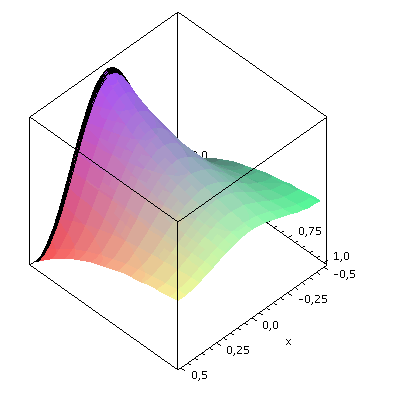
> p10:=smod:-plot3d(t=0..1,x=-0.5..0.5,style=patchnogrid):

> p11:=smod:-plot3d(t=0..0.02,x=-0.5..0.5):

> plots[display]({p11, p10},axes=boxed,axis[1,2]=[mode=linear]);